Observations¶

For all environments, several types of observations can be used. They are defined in the observation module. Each environment comes with a default observation, which can be changed or customised using environment configurations. For instance,

import gymnasium as gym
import highway_env

env = gym.make(
    'highway-v0',
    config={
        "observation": {
            "type": "OccupancyGrid",
            "vehicles_count": 15,
            "features": ["presence", "x", "y", "vx", "vy", "cos_h", "sin_h"],
            "features_range": {
                "x": [-100, 100],
                "y": [-100, 100],
                "vx": [-20, 20],
                "vy": [-20, 20]
            },
            "grid_size": [[-27.5, 27.5], [-27.5, 27.5]],
            "grid_step": [5, 5],
            "absolute": False
        }
    }
)
env.reset()

Note

The "type" field in the observation configuration takes values defined in observation_factory() (see source)

Kinematics¶

The KinematicObservation is a \(V\times F\) array that describes a list of \(V\) nearby vehicles by a set of features of size \(F\), listed in the "features" configuration field. For instance:

Vehicle	\(x\)	\(y\)	\(v_x\)	\(v_y\)
ego-vehicle	5.0	4.0	15.0	0
vehicle 1	-10.0	4.0	12.0	0
vehicle 2	13.0	8.0	13.5	0
…	…	…	…	…
vehicle V	22.2	10.5	18.0	0.5

Note

The ego-vehicle is always described in the first row

If configured with normalize=True (default), the observation is normalized within a fixed range, which gives for the range [100, 100, 20, 20]:

Vehicle	\(x\)	\(y\)	\(v_x\)	\(v_y\)
ego-vehicle	0.05	0.04	0.75	0
vehicle 1	-0.1	0.04	0.6	0
vehicle 2	0.13	0.08	0.675	0
…	…	…	…	…
vehicle V	0.222	0.105	0.9	0.025

If configured with absolute=False, the coordinates are relative to the ego-vehicle, except for the ego-vehicle which stays absolute.

Vehicle	\(x\)	\(y\)	\(v_x\)	\(v_y\)
ego-vehicle	0.05	0.04	0.75	0
vehicle 1	-0.15	0	-0.15	0
vehicle 2	0.08	0.04	-0.075	0
…	…	…	…	…
vehicle V	0.172	0.065	0.15	0.025

Note

The number \(V\) of vehicles is constant and configured by the vehicles_count field, so that the observation has a fixed size. If fewer vehicles than vehicles_count are observed, the last rows are placeholders filled with zeros. The presence feature can be used to detect such cases, since it is set to 1 for any observed vehicle and 0 for placeholders.

Feature	Description
\(presence\)	Disambiguate agents at 0 offset from non-existent agents.
\(x\)	World offset of ego vehicle or offset to ego vehicle on the x axis.
\(y\)	World offset of ego vehicle or offset to ego vehicle on the y axis.
\(vx\)	Velocity on the x axis of vehicle.
\(vy\)	Velocity on the y axis of vehicle.
\(heading\)	Heading of vehicle in radians.
\(cos_h\)	Trigonometric heading of vehicle.
\(sin_h\)	Trigonometric heading of vehicle.
\(cos_d\)	Trigonometric direction to the vehicle’s destination.
\(sin_d\)	Trigonometric direction to the vehicle’s destination.
\(long_{off}\)	Longitudinal offset to closest lane.
\(lat_{off}\)	Lateral offset to closest lane.
\(ang_{off}\)	Angular offset to closest lane.

Example configuration¶

import gymnasium as gym
import highway_env

config = {
    "observation": {
        "type": "Kinematics",
        "vehicles_count": 15,
        "features": ["presence", "x", "y", "vx", "vy", "cos_h", "sin_h"],
        "features_range": {
            "x": [-100, 100],
            "y": [-100, 100],
            "vx": [-20, 20],
            "vy": [-20, 20]
        },
        "absolute": False,
        "order": "sorted"
    }
}
env = gym.make('highway-v0', config=config)
obs, info = env.reset()
print(obs)

[[ 1.          1.          0.12        1.          0.          1.
   0.        ]
 [ 1.          0.20796539  0.         -0.07930574  0.          1.
   0.        ]
 [ 1.          0.43728748  0.         -0.10441518  0.          1.
   0.        ]
 [ 1.          0.63276297  0.         -0.16635698  0.          1.
   0.        ]
 [ 1.          0.8445503  -0.12       -0.10898441  0.          1.
   0.        ]
 [ 1.          1.         -0.12       -0.12598878  0.          1.
   0.        ]
 [ 1.          1.         -0.04       -0.07915984  0.          1.
   0.        ]
 [ 1.          1.         -0.12       -0.1142595   0.          1.
   0.        ]
 [ 1.          1.         -0.08       -0.11307526  0.          1.
   0.        ]
 [ 1.          1.         -0.04       -0.16392277  0.          1.
   0.        ]
 [ 0.          0.          0.          0.          0.          0.
   0.        ]
 [ 0.          0.          0.          0.          0.          0.
   0.        ]
 [ 0.          0.          0.          0.          0.          0.
   0.        ]
 [ 0.          0.          0.          0.          0.          0.
   0.        ]
 [ 0.          0.          0.          0.          0.          0.
   0.        ]]

Grayscale Image¶

The GrayscaleObservation is a \(W\times H\) grayscale image of the scene, where \(W,H\) are set with the observation_shape parameter. The RGB to grayscale conversion is a weighted sum, configured by the weights parameter. Several images can be stacked with the stack_size parameter, as is customary with image observations.

Example configuration¶

from matplotlib import pyplot as plt
%matplotlib inline
config = {
    "observation": {
        "type": "GrayscaleObservation",
        "observation_shape": (128, 64),
        "stack_size": 4,
        "weights": [0.2989, 0.5870, 0.1140],  # weights for RGB conversion
        "scaling": 1.75,
    },
    "policy_frequency": 2
}
env = gym.make('highway-v0', config=config)
obs, info = env.reset()

fig, axes = plt.subplots(ncols=4, figsize=(12, 5))
for i, ax in enumerate(axes.flat):
    ax.imshow(obs[i, ...].T, cmap=plt.get_cmap('gray'))
plt.show()

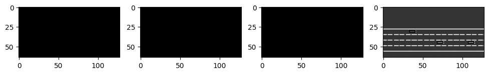
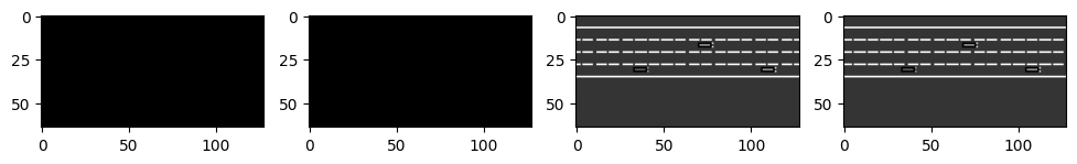
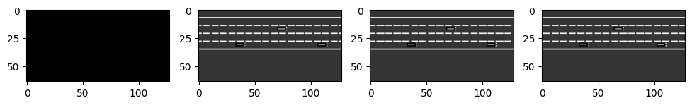
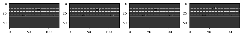
Illustration of the stack mechanism¶

We illustrate the stack update by performing three steps in the environment.

for _ in range(3):
    obs, reward, done, truncated, info = env.step(env.unwrapped.action_type.actions_indexes["IDLE"])

    fig, axes = plt.subplots(ncols=4, figsize=(12, 5))
    for i, ax in enumerate(axes.flat):
        ax.imshow(obs[i, ...].T, cmap=plt.get_cmap('gray'))
plt.show()

Occupancy grid¶

The OccupancyGridObservation is a \(W\times H\times F\) array, that represents a grid of shape \(W\times H\) discretising the space \((X,Y)\) around the ego-vehicle in uniform rectangle cells. Each cell is described by \(F\) features, listed in the "features" configuration field. The grid size and resolution is defined by the grid_size and grid_steps configuration fields.

For instance, the channel corresponding to the presence feature may look like this:

presence feature: one vehicle is close to the north, and one is farther to the east.¶
0	0	0	0	0
0	0	1	0	0
0	0	0	0	1
0	0	0	0	0
0	0	0	0	0

The corresponding \(v_x\) feature may look like this:

\(v_x\) feature: the north vehicle drives at the same speed as the ego-vehicle, and the east vehicle a bit slower¶
0	0	0	0	0
0	0	0	0	0
0	0	0	0	-0.1
0	0	0	0	0
0	0	0	0	0

Example configuration¶

"observation": {
    "type": "OccupancyGrid",
    "vehicles_count": 15,
    "features": ["presence", "x", "y", "vx", "vy", "cos_h", "sin_h"],
    "features_range": {
        "x": [-100, 100],
        "y": [-100, 100],
        "vx": [-20, 20],
        "vy": [-20, 20]
    },
    "grid_size": [[-27.5, 27.5], [-27.5, 27.5]],
    "grid_step": [5, 5],
    "absolute": False
}

Time to collision¶

The TimeToCollisionObservation is a \(V\times L\times H\) array, that represents the predicted time-to-collision of observed vehicles on the same road as the ego-vehicle. These predictions are performed for \(V\) different values of the ego-vehicle speed, \(L\) lanes on the road around the current lane, and represented as one-hot encodings over \(H\) discretised time values (bins), with 1s steps.

For instance, consider a vehicle at 25m on the right-lane of the ego-vehicle and driving at 15 m/s. Using \(V=3,\, L = 3\,H = 10\), with ego-speed of {\(15\) m/s, \(20\) m/s and \(25\) m/s}, the predicted time-to-collisions are \(\infty,\,5s,\,2.5s\) and the corresponding observation is

0	0	0	0	0	0	0	0	0	0
0	0	0	0	0	0	0	0	0	0
0	0	0	0	0	0	0	0	0	0

0	0	0	0	0	0	0	0	0	0
0	0	0	0	0	0	0	0	0	0
0	0	0	0	1	0	0	0	0	0

0	0	0	0	0	0	0	0	0	0
0	0	0	0	0	0	0	0	0	0
0	0	1	0	0	0	0	0	0	0

The top row corresponds to the left-lane, the middle row corresponds to the lane where ego-vehicle is located, and the bottom row to the right-lane.

Example configuration¶

"observation": {
    "type": "TimeToCollision"
    "horizon": 10
},

Lidar¶

The LidarObservation divides the space around the vehicle into angular sectors, and returns an array with one row per angular sector and two columns:

distance to the nearest collidable object (vehicles or obstacles)
component of the objects’s relative velocity along that direction

The angular sector of index 0 corresponds to an angle 0 (east), and then each index/sector increases the angle (south, west, north).

For example, for a grid of 8 cells, an obstacle 10 meters away in the south and moving towards the north at 1m/s would lead to the following observation:

the Lidar observation¶
0	0
0	0
10	-1
0	0
0	0
0	0
0	0
0	0

Here is an example of what the distance grid may look like in the parking env:

env = gym.make(
    'parking-v0',
    render_mode='rgb_array',
    config={
        "observation": {
            "type": "LidarObservation",
            "cells": 128,
        },
        "vehicles_count": 3,
    })
env.reset()

plt.imshow(env.render())
plt.show()

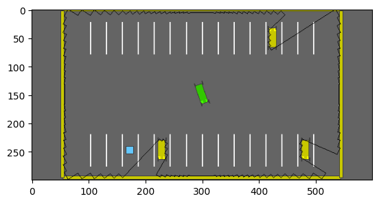
You can configure the number of cells in the angular grid with the cells parameter, the maximum range with maximum_range, and if you enable normalize, then distances and relative speeds are both divided by the maximum range.

Example configuration¶

"observation": {
    "type": "LidarObservation",
    "cells": 128,
    "maximum_range": 64,
    "normalise": True,
}

API¶

class highway_env.envs.common.observation.GrayscaleObservation(env: AbstractEnv, observation_shape: tuple[int, int], stack_size: int, weights: list[float], scaling: float | None = None, centering_position: list[float] | None = None, **kwargs)[source]¶

An observation class that collects directly what the simulator renders.

Also stacks the collected frames as in the nature DQN. The observation shape is C x W x H.

Specific keys are expected in the configuration dictionary passed. Example of observation dictionary in the environment config:

observation”: {
“type”: “GrayscaleObservation”, “observation_shape”: (84, 84) “stack_size”: 4, “weights”: [0.2989, 0.5870, 0.1140], # weights for RGB conversion,

}

space() → Space[source]¶: Get the observation space.

observe() → ndarray[source]¶: Get an observation of the environment state.

class highway_env.envs.common.observation.KinematicObservation(env: AbstractEnv, features: list[str] = None, vehicles_count: int = 5, features_range: dict[str, list[float]] = None, absolute: bool = False, order: str = 'sorted', normalize: bool = True, clip: bool = True, see_behind: bool = False, observe_intentions: bool = False, include_obstacles: bool = True, **kwargs: dict)[source]¶

Observe the kinematics of nearby vehicles.

Parameters:

env – The environment to observe
features – Names of features used in the observation
vehicles_count – Number of observed vehicles
features_range – a dict mapping a feature name to [min, max] values
absolute – Use absolute coordinates
order – Order of observed vehicles. Values: sorted, shuffled
normalize – Should the observation be normalized
clip – Should the value be clipped in the desired range
see_behind – Should the observation contains the vehicles behind
observe_intentions – Observe the destinations of other vehicles

space() → Space[source]¶: Get the observation space.

normalize_obs(df: DataFrame) → DataFrame[source]¶

Normalize the observation values.

For now, assume that the road is straight along the x axis. :param Dataframe df: observation data

observe() → ndarray[source]¶: Get an observation of the environment state.

class highway_env.envs.common.observation.OccupancyGridObservation(env: AbstractEnv, features: list[str] | None = None, grid_size: tuple[tuple[float, float], tuple[float, float]] | None = None, grid_step: tuple[float, float] | None = None, features_range: dict[str, list[float]] = None, absolute: bool = False, align_to_vehicle_axes: bool = False, clip: bool = True, as_image: bool = False, **kwargs: dict)[source]¶

Observe an occupancy grid of nearby vehicles.

Parameters:

env – The environment to observe
features – Names of features used in the observation
grid_size – real world size of the grid [[min_x, max_x], [min_y, max_y]]
grid_step – steps between two cells of the grid [step_x, step_y]
features_range – a dict mapping a feature name to [min, max] values
absolute – use absolute or relative coordinates
align_to_vehicle_axes – if True, the grid axes are aligned with vehicle axes. Else, they are aligned with world axes.
clip – clip the observation in [-1, 1]

space() → Space[source]¶: Get the observation space.

normalize(df: DataFrame) → DataFrame[source]¶

Normalize the observation values.

For now, assume that the road is straight along the x axis. :param Dataframe df: observation data

observe() → ndarray[source]¶: Get an observation of the environment state.

pos_to_index(position: ndarray | Sequence[float], relative: bool = False) → tuple[int, int][source]¶

Convert a world position to a grid cell index

If align_to_vehicle_axes the cells are in the vehicle’s frame, otherwise in the world frame.

Parameters:

position – a world position
relative – whether the position is already relative to the observer’s position

Returns:

the pair (i,j) of the cell index

fill_road_layer_by_lanes(layer_index: int, lane_perception_distance: float = 100) → None[source]¶

A layer to encode the onroad (1) / offroad (0) information

Here, we iterate over lanes and regularly placed waypoints on these lanes to fill the corresponding cells. This approach is faster if the grid is large and the road network is small.

Parameters:

layer_index – index of the layer in the grid
lane_perception_distance – lanes are rendered +/- this distance from vehicle location

fill_road_layer_by_cell(layer_index) → None[source]¶

A layer to encode the onroad (1) / offroad (0) information

In this implementation, we iterate the grid cells and check whether the corresponding world position at the center of the cell is onroad/offroad. This approach is faster if the grid is small and the road network large.

class highway_env.envs.common.observation.KinematicsGoalObservation(env: AbstractEnv, scales: list[float], **kwargs: dict)[source]¶

Parameters:

env – The environment to observe
features – Names of features used in the observation
vehicles_count – Number of observed vehicles
features_range – a dict mapping a feature name to [min, max] values
absolute – Use absolute coordinates
order – Order of observed vehicles. Values: sorted, shuffled
normalize – Should the observation be normalized
clip – Should the value be clipped in the desired range
see_behind – Should the observation contains the vehicles behind
observe_intentions – Observe the destinations of other vehicles

space() → Space[source]¶: Get the observation space.

observe() → dict[str, ndarray][source]¶: Get an observation of the environment state.

class highway_env.envs.common.observation.ExitObservation(env: AbstractEnv, features: list[str] = None, vehicles_count: int = 5, features_range: dict[str, list[float]] = None, absolute: bool = False, order: str = 'sorted', normalize: bool = True, clip: bool = True, see_behind: bool = False, observe_intentions: bool = False, include_obstacles: bool = True, **kwargs: dict)[source]¶

Specific to exit_env, observe the distance to the next exit lane as part of a KinematicObservation.

Parameters:

env – The environment to observe
features – Names of features used in the observation
vehicles_count – Number of observed vehicles
features_range – a dict mapping a feature name to [min, max] values
absolute – Use absolute coordinates
order – Order of observed vehicles. Values: sorted, shuffled
normalize – Should the observation be normalized
clip – Should the value be clipped in the desired range
see_behind – Should the observation contains the vehicles behind
observe_intentions – Observe the destinations of other vehicles

observe() → ndarray[source]¶: Get an observation of the environment state.